From the first moments this observer gazed into the night sky with a telescope it was apparent that our atmosphere was anything but crystal clear. The Earth’s sky is not completely transparent and as stable as we would like it to be. Experienced observers are well aware that turbulent air currents can cause telescopic images to blur or move around in the eyepiece field. Since the Earth’s atmosphere acts like a fluid, we may think of it as a very thin body of water. Imagine yourself at the bottom of a clear lake looking up at the Moon! We have coined the phrase, "astronomical seeing," to quantify, or put into perspective, the effect the atmosphere has on image quality.

Bad seeing can render a night’s observing schedule useless, especially for us planet watchers. Even though seeing conditions may improve for brief moments during periods bad seeing, we should pay attention to weather reports. Just because a weather forecast calls for clear sky that does not mean the atmosphere will be good for observing.

None of this should be a surprise to anyone who has peered through a telescope, even at the Moon. At times, the Moon appears like it swimming in water or above a smokestack! Our atmosphere makes observing Solar System objects nearly impossible at times. The words of a great Mars observer, Gerard de Vaucouleurs from his book, The Planet Mars, say it all:

"It is no exaggeration to say that if, in summer, we look at the Moon when it is just rising above the level of a tarred road that has been warmed by the Sun all day, we shall get a good picture of the conditions under which observers of Mars generally find themselves."

Streams of warm and cold air mixing and flowing together will cause atmospheric turbulence. Most of the disruptive atmospheric turbulence occurs very near the Earth’s surface up to around 50,000 feet. Above this altitude, the atmosphere begins to thin out and the airflow, or winds, tends to be in the same direction with each other -- therefore reducing the effects of turbulent cross winds or violent updrafts. In other words, the higher the altitude the steadier the airflow is.

The jet stream is a belt or band of rapidly moving air from 50,000 feet in altitude, or above, crossing the mid-latitudes of the U.S. Actually, there are two jet streams. One in the far northern U.S. and Canada and the other moves north or south across the center of our country. The jet stream tends to change in latitude seasonally and will meander across the country like a river of turbulent water.

The air at altitudes above or below the jet stream may be calm and flowing steadily in one direction, but the jet stream does not always flow the same path as the surrounding airflow. Crosswords or vertical wind in this circumstance causes a decrease in "seeing." Also, the southern edge of the jet stream will often contain ice formations or cirrus clouds that tend to help seeing at times and hinder it at other times. Irregular, disturbed cirrus clouds are not good. Cirrus clouds, or "mare’s tails" as they are often referred to, are usually uniform streaks indicating smooth airflow. However, the clear region just north of this band of cirrus clouds may be very turbulent.

These air streams or "thermal currents" causes apparent starlight to change directions and intensity. Because the density of air varies with temperature and the refractive index of air depends on the density of air, starlight does not traverse through it without interference. Thermal currents in the air have a similar effect as if there were thousands of lenses floating around in it.

Atmospheric thermal currents also vary the amount of starlight passing through it and we call this atmospheric "extinction." Random intensity fluctuations of starlight passing through the atmosphere are called "scintillation." You can easily see the effects of scintillation by looking up at night right after a cold front and see the star twinkle and change colors. Refraction within the thermal cells also causes the color of the object to rapidly change.   The altitude or elevation about the horizon also effects astronomical seeing due to the increase in airmass.

Air pollution also affects seeing. Seeing in large industrial areas will have several types of particles and dust materials circulating at lower altitudes. These particles store heat and will cause thermal air currents. The largest polluters are not manmade though; volcanoes are known to wreck havoc on astronomical seeing. Starting with the irruption of Mt. St. Helens (northwestern U.S.A.) in the early 1980’s, El Chichon (Mexico) sometime later, and the recent Penetubo (Philippines) irruption in 1991, we see how these natural phenomena can restrict our sky watching in the equatorial regions of Earth. That deep red sky at twilight may be beautiful; however, this indicates that the upper atmosphere is full of particles that disrupt the air flows and effects seeing. These dust particles fall to Earth in short order; however, several active chemical compounds remain in the upper atmosphere for months, even years, to reduce transparency and seeing.

Dust storms in the African deserts can also cause seeing problems in some parts of the southeastern United States. When this occurs a dusty haze covers the entire sky for weeks and seeing goes right down the tube, so to speak.

All of the above conditions cause starlight to oscillate about the sky, or "twinkle," and blur, thereby causing them to appear larger than they really are. In smaller telescopes these fluctuations appears to shift star images around or make the entire planetary images to oscillate. In larger instruments, the image tends to blur or smear.

In the case of the small instruments the apparent size of these "seeing cells," or "thermal currents," are closer to the same size as the apparent angle of the object we see at the telescopes focal plane. However, in larger instruments the angular image size is larger so these same "seeing cells" and disrupt different areas within the image. So the planet image may expand and contract or blur.

There is some dispute in the scientific community as to what constitutes a major contributor to air pollution. Some declare the Earth is in eminent peril due to Man’s machinery and others say this not so. To those who discount the extent to what volcanic eruptions or African dust storms can or can’t do to our atmosphere should go out and look up sometimes. Maybe look up with a telescope!

In the past several experienced planetary observers complained to me about their bad seeing at their home. At the time there was no reason to doubt these observers it occurred to me to ask where their telescope was setup for observing. Inevitably they would tell me their telescope would usually be rolled out of a garage onto an asphalt driveway to observe. This is probably the worst surface to setup a telescope on because after it begins to cool off after dark heat will boil up for the surface for hours on end. When I advised them to just move off into the grass and after they tired it their complaining of bad seeing went away.

For most of our lives we have little choice in selecting an observing site. We must provide for our family and go where the jobs are, find available of housing, shopping, transportation, etc., and this usually means living in large metropolitan areas. Even if our choices are limited we can usually make our home a better place to observe from by following a few rules in studying micrometeorology. This deals with the atmosphere a few yards above the ground. A study of our neighborhood is important in determining what obstructions are close by that will cause turbulence about our telescopes.

Micrometeorology is the study of the atmosphere from the surface up to a few yards (See NOTE 1). Since we cannot do much about the atmosphere, we do have some control over where we locate our observing site. The Earth’s atmosphere is composed of gases, mostly nitrogen, oxygen -- and water vapor -- and it is not invisible ( Munn, 1966].

Gaseous vapors have mass and at times may feel like a fluid; especially in South Florida were the humidity reaches nearly 100% at times. Humidity is a measure of how much moisture is in the air and indicates at what point the air will become foggy or hazy. Meteorologists call this point or condition the "dew point."

Nearer to the Earth’s surface there are obstructions, such as mountains, hills, lakes, trees, buildings, etc., that disrupts the air flow and is a major cause of bad seeing. Yes, even trees can effect seeing and some more than others. We will discuss this later.

When planning an observing site it is important to select high ground if possible. Airflow is less turbulent over hills than in valleys. In addition, observing from the lee side of a lake can be interesting (the lee side is where wind blows over the water to you). Seeing conditions are definitely better on lee side of the lake or seacoast where the airflow tends to be nearly saturated and more often will cause a temperature inversion over the coastal areas. When this condition occurs a ground fog will begin over the land and causes the air above to be less turbulent. However, the air flowing from dry land tends to more turbulent.

Air circulation over the ocean and shorelines in coastal areas is very complex and defies a simple or brief explanation here. However, well known to those living near coastal areas is that astronomical seeing can be excellent, at times providing the best conditions for telescopic viewing. Conditions near the coast changes dramatically with the seasons too. This is another very complex subject and will be omitted as well.

The same thing occurs near buildings that happen to be near lakes or mountains. The wind may not blow your telescope around as much behind the house, but seeing will suffer. The peaked roof and heat rising from the house causes turbulent down drafts that spoils the air flow over your telescope. Move your telescope to the other side, away from the "lee" side and seeing improves.

Trees will radiate heat and emit vapors at nightfall, therefore spoiling the air immediately above them. Pine trees are among the worst offenders and this writer avoids setting up a telescope in a densely populated pine forest. The problem in forests is not quite, as simple as previously stated. The main force that disrupts the air above the forest comes from vertical air circulation within the trees. Also, in pine forests the thick layer of the heat storing biomoss (dead pine needles) releases heat plumes after the Sun sets. Combined with the up and down airflow this heat causes much turbulence over the trees. However, not all is lost for tree dwellers. A forest may be beneficial to daytime telescopic observing. It is well know among glider pilots that air above a forest is calm during day time, giving rise to the suggestion that seeing may be good during the daylight hours over these trees.

NOTE: Boundary Layer - In general, a layer of air adjacent to a bounding surface. Specifically, the term most often refers to the planetary boundary layer, which is the layer within which the effects of friction are significant. For the earth, this layer is considered to be roughly the lowest one or two kilometers of the atmosphere. It is within this layer that temperatures are most strongly affected by daytime insolation and nighttime radiational cooling, and winds are affected by friction with the earth’s surface. The effects of friction die out gradually with height, so the "top" of this layer cannot be defined exactly.

There is a thin layer immediately above the earth’s surface known as the surface boundary layer (or simply the surface layer). This layer is only a part of the planetary boundary layer, and represents the layer within which friction effects are more or less constant throughout (as opposed to decreasing with height, as they do above it). The surface boundary layer is roughly 10 meters thick, but again the exact depth is indeterminate. Like friction, the effects of insolation and radiational cooling are strongest within this layer.

Intereting Internet Sites:

Atmospheric Seeing on Wikipedia:   http://en.wikipedia.org/wiki/Astronomical_seeing
Damian Peach (Scales):   http://www.damianpeach.com/pickering.htm
Damian Peach (Planet) : http://www.damianpeach.com/seeing1.htm
Damian Peach (A guide to Astronomical seeing):  http://www.cloudynights.com/item.php?item_id=555
Meteoblue>Outdoor and Sports>Astronomical Seeing: : https://www.meteoblue.com/en/weather/outdoorsports/seeing/
Seeing Observations Database :   http://cleardarksky.com/so/
Understanding Atmospheric Seeing:     http://home.no.net/jonbent/Sky.html
Weather Forecast for  Astronomy:  http://weatheroffice.ec.gc.ca/astro/index_e.html
 
 

Over the years visual observers have derived many schemes to describe "astronomical seeing" in a quantitative manner. First, the scales used by many in the Association of Lunar and Planetary Observers (A.L.P.O.).

An A.L.P.O. Scale: The first step is to determine the observer’s "personal constant" by using several double stars on a "night of exceptional seeing," and with the aperture stopped down to 1 inch. This "personal constant, r, is the separation in seconds of arc of the closest pair which can barely be separated.

Step two: This requires that, on a night of actual observing, the observer find the closest double star, which can be resolved, using the full aperture and then multiply that separation by the aperture in inches, yielding a value r’ . This is used along with r (as found above) to calculate the telescope efficiency, e , as: e = r / r’

Modification of Step One above: the observer would perhaps be better served by using the methodology described by Couteau in Chapter 4 of Observing Visual Double Stars where he explains in detail how to use artificial lighting and small ball bearings to create artificial double stars located some distance away from the observer. In his own words (p. 89):
 

"You will have a stable stellar image, unaffected by seeing, that can easily be examined comfortably, without twisting your neck. Reflections from two lamps, side by side, will give a beautiful double star. The separation can be varied at will, up to the limit of resolution, and even differences in brightness can be created by moving one lamp with respect to the other."

By using the formula Couteau provides, all variables (ball bearing radius, distance between the lamps, distance from lamps to ball bearing, and distance from telescope objective to ball bearing) are used to define the separation of the artificial pair in arc seconds. In his example, he uses a 4mm ball bearing, lamps separated by 10cm and located 1m from the bearing, and an observer 100m away, to yield a 0.2 arc second separation.

A suitable "test stand" could be built to allow the "personal constant" to be determined without regard to whether or not it was a "night of exceptional seeing." Such a test stand could also be used to compare telescopes of the same aperture to determine which had the better absolute resolution.

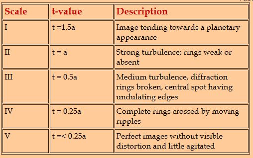
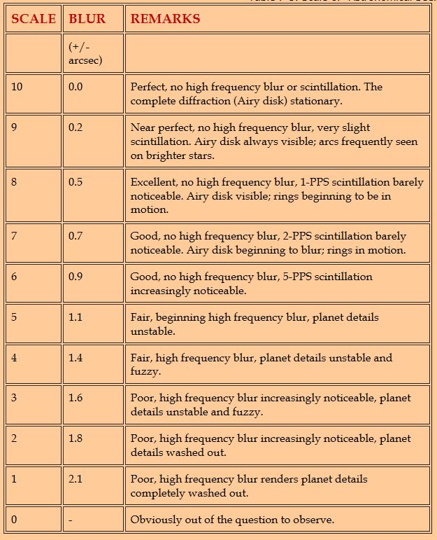
In Texeraux’s How to make a Telescope, Willman-Bell, 2nd ed, p309-310) and Jean Dragesco’s High Resolution Astrophotography , CUP, p3-4) and noted the following quantitative scale to estimate seeing based on the work of Danjon and Couder (1935). It also gets a mention in Sidgwick’s Amateur Astronomer’s Handbook , 2nd ed, p454-455). This scale provides an absolute notion of seeing expressed in arc seconds and is not tied to any specific aperture, unlike some of the other scales in common use e.g. Antoniadi. We may assume the Rayleigh limit (140/Dmm) as the baseline measure. In use one simply compares the degree of turbulence in the Airy pattern with the description, and then reads off the value.

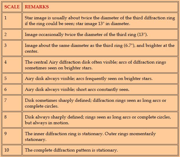
Another scale: Harvard Observatory’s William H. Pickering (1858-1938). Pickering used a 5-inch refractor. His comments about diffraction disks and rings will have to be modified for larger or smaller instruments, but they’re a starting point:

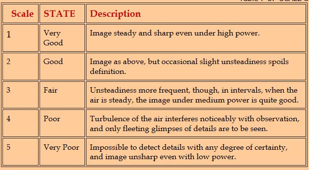
Yet another scale: Another system of measuring “astronomical seeing” can be found in the translated version (translated by Alex Helm) of the Handbook for Planetary Observers ,  by: Gunter D. Roth, Van Nostrand Reinhold Company, New York, 1970 edition (No ISDN identification can be found in this handbook).  This book is out of print and very hard to find.

In his chapter, “Assessing the state of the atmosphere,”  Roth discusses the importance of keeping records of observations and recording the atmospheric conditions during the observational period.  He talks about the attempts to produce a usable seeing scale and the difficulties in such a feat.  More importantly he points out, “that one cannot really compare conditions in terms of a 10-inch telescope on the one hand, and a 3-inch on the other.” This is quite obvious to those experienced observers who use a variety of telescopes; however, many a novice observer may miss this fact and this author has witnessed confusion in inexperienced observers many times over this issue.   Included in the handbook is his treatment of “astronomical seeing” and he tabulates his perceptions in the table below.  Scale of  “Assessing the state of the atmosphere” from Handbook for Planetary Observers.

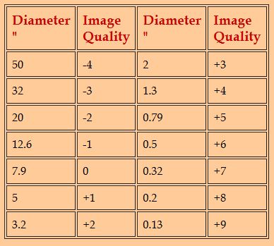
He continues with how aperture and apparent size of he object under study also can effect out perceptions of seeing. He gives an example of studies by O. R. Norton of the University of Nevada whereby he concludes that the apparent effect of atmospheric turbulence has a lesser effect on seeing by using a smaller telescope aperture.  This has been a matter of many debates.  More importantly he points out that the radius of the shimmering of the image in a telescope should be taken as a measure of the atmospheric conditions.

Norton continues,  “The diameter of the shimmering disc can be estimated fairly easily by means of the distance between components of a double star pair.”  Roth then included a table that was compiled by Clyde Tombaugh and B.A. Smith” and is tabulated in the below.   Scale of  “Assessing the state of the atmosphere” from Handbook for Planetary Observers.

After surveying many astronomical books surfing the Net looking for reports on "astronomical seeing" it is obvious the subject lacks credible description. These is a paper trail talking points on the subject, however, a detail description is limited to what amateur astronomers have to say. One may wish to use modern photometers, electronics and computers to record intensities variations of stars, but that would be too much like work. Someday it would be nice if someone would describe in empirical terms "astronomical seeing."

Micrometer Seeing Scale:   This author has used a Bi-filar micrometer on many occasions to measure the blurring and slow expansion and contraction of Mars to convert to angles and compare those results with well known seeing scales. By calculating the linear or plate scale of the telescope (using the focal length and eyepiece apparent angles) one can then measure the amount of displacement in the image in seconds of arc. This can then be applied to the definitions of the various seeing scales. My personal seeing scale is a number between 0 and 10 that is defined as follows:

So, the above demonstrates just how subjective the published and unpublished "astronomical seeing" scales can be. The time and effort to make our personal reference to astronomical seeing more scientific is worth while for an observer to do occasionally. But, it is not necessary to conduct testing at each observation period. Experienced planetary observers will on occasion test his or her "personal equation." That includes some measure of what they perceive the "seeing" to be.  Subjectivity is just a human perception. Remember, after all the high tech- machines record minute data points and statistical curves and tables, it is the human eye that renders science a subjective art for the human mind.

More seeing scales have been published over the years and if anyone else can add to this list please do. Maybe reduce the confusion of the seeing scales to one everyone can understand.

While this paper covered several aspects of “astronomical seeing,” the transparency scale that is often asked for in A.L.P.O. or B.A.A. observational forms is seldom mentioned in detail.  Most often transparency is simply described as the measure of how clear the sky is. By looking for the faintest star in the sky and fitting this to some arbitrary scale we satisfy this criteria. Some A.L.P.O. sections use a transparency of 1 to 6, or the faintest star detectable from; 1st magnitude through 6th., where the latter is near the lower threshold of the human sight.

Transparency is a measure of the clarity of the air.  Haze, smoke, dust particles will reduce the clarity of out atmospheres and can be readily seen in and around brightly lit cities and a general background glow. A 6th magnitude star out in the darker countryside may not be visible in the city.  One may not even detect 4th or 5th magnitude stars in the city because of the background glow of “light pollution.”  Light pollution can light up particles suspended in the atmosphere up to thousands of feet.  Clouds can bee seen to glow even above 6,000 feet altitude.   Regions with high humidity can also effect transparency, especially in the red end of the spectrum.

In this chapter, ‘Astronomical Seeing’ and ‘Astronomical Seeing’ Scales, we now have a good foundation for describing in quantitative terms the seeing conditions for an observing site and time period. It can be a bit confusing when attempting to state the seeing conditions on observational report forms and each ALPO section has their own methods and requirments. So, one must consult the section leaders as to their desires. Most sections use a typical seeing scale using 0 to 10, where 0 is very bad seeing to a perfect 10.

One must also consider what trees, houses, lakes, mountains, and other obstructions near the the observer’s site effects his or her "astronomical seeing." Another very important ingredient in this saga is tube currents within the observers telescope and surface heat currents from an equatorial mount, a concrete pad or asphalt driveway. An observer may be fooled for years into believing his sky conditions are the cause of the bad seeing when it could be as simple as a badly designed telescope tube or where the telescope sits on the ground. This is a subject for a follow up article and wouldn’t it be great if a member of one of our Electronic ALPO submit an article on just this topic?

South and Central Florida provides us with some interesting conditions to observe in and you can read about it here: Florida_Seeing.html

For an advanced course in “astronomical seeing” and transparency,  Sidgwick’s Amateur Astronomer’s Handbook, chapter  26, “The Atmosphere and Seeing,” starting on page 445,  describes these factors in great detail.  Another more advanced dissertation can be found in a chapter, “The Theory of Visual Lunar and Planetary Observation,” in the A.L.P.O. book Observing the Moon, Planets, and Comets, by: Clark Chapman and Dale Cruikshank  Also, see Dobbins, T.A., D.C. Parker, and C.F. Capen, Introduction to Observing and Photographing the Solar System, Chapter 7.1.4, pp. 57. Willmann-Bell, Inc., Richmond.

A comprehensive and detailed synopsis of "Astronomical Seeing" can be found in the following links:

Astronomical Seeing; Part 1: The Nature of Turbulence:

Astronomical Seeing; Part 2: Seeing Measurement Methods:

Astronomical Seeing; Part 3: Observing Techniques:

However, for most observers a more general statement and definition can be found in Phil Harrington’s, Star Ware, Chapter 9, beginning on page 241 and Michael Porcellino’s Through the Telescope,  Chapter 7,  page 101, “Transparency.”